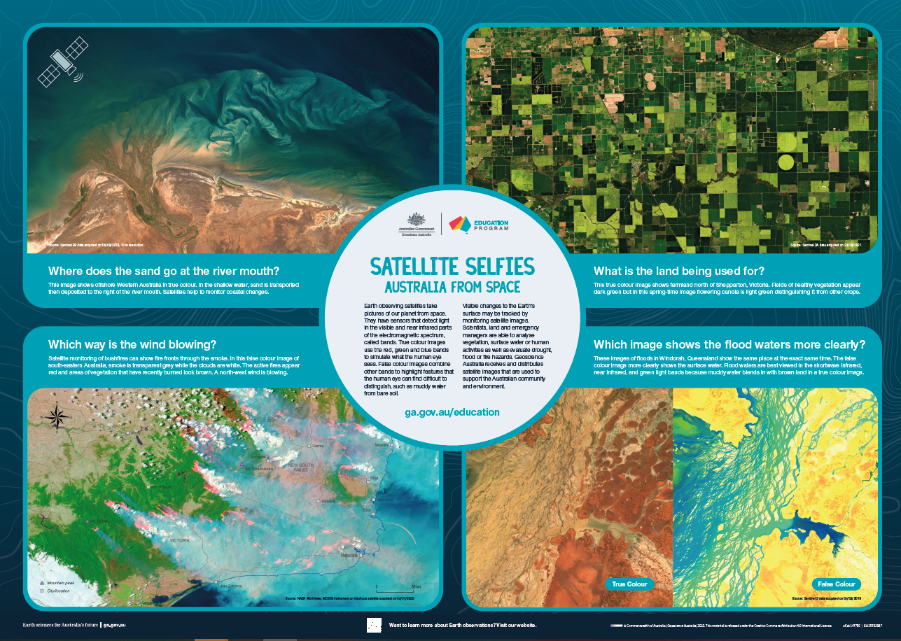
<div>The A1 poster incorporates 4 images of Australia taken from space by Earth observing satellites. The accompanying text briefly introduces sensors and the bands within the electromagnetic spectrum. The images include examples of both true and false colour and the diverse range of applications of satellite images such as tracking visible changes to the Earth’s surface like crop growth, bushfires, coastal changes and floods. Scientists, land and emergency managers use satellite images to analyse vegetation, surface water or human activities as well as evaluate natural&nbsp;hazards.</div>

User Manual - Australian Flood Studies Database Search

Floods are Australia's most expensive natural hazard with the average annual cost of floods estimated at AUD$377 million (BITRE 2008). This figure is likely to have risen following the widespread and devastating floods across eastern Australia that occurred over the summer of 2010-11. The development of tools to support the identification and analysis of flood risk is an important first step in reducing the cost of floods in the community. The Australian Government through Geoscience Australia (GA) has been leading the development of tools which assist in flood intelligence, modelling and damage assessment. An overview of three of these tools will be provided in this presentation. Note: Rest of abstract is too long for space provided.

<div>Groundwater dependent ecosystems (GDEs) rely on access to groundwater on a permanent or intermittent basis to meet some or all of their water requirements (Richardson et al., 2011). The <a href="https://explorer-aws.dea.ga.gov.au/products/ga_ls_tc_pc_cyear_3">Tasselled Cap percentile products</a> created by Digital Earth Australia (2023) were used to identify potential GDEs for the upper Darling River floodplain study area. These percentile products provide statistical summaries (10th, 50th, 90th percentiles) of landscape brightness, greenness and wetness in imagery acquired between 1987 and present day. The 10th percentile greenness and wetness represent the lowest 10% of values for the time period evaluated, e.g. 10th greenness represents the least green period. In arid regions, areas that are depicted as persistently green and/or wet at the 10th percentile have the greatest potential to be GDEs. For this reason, and due to accessibility of the data, the 10th percentile Tasselled Cap greenness (TCG) and Tasselled Cap wetness (TCW) products were used as the basis for the assessment of GDEs for the upper Darling River floodplain study area. </div><div><br></div><div>This data release is an ESRI geodatabase, with layer files, including:</div><div><br></div><div>-&nbsp;&nbsp;&nbsp;&nbsp;&nbsp;&nbsp;original greenness and wetness datasets extracted; </div><div><br></div><div>-&nbsp;&nbsp;&nbsp;&nbsp;&nbsp;&nbsp;classified 10th percentile greenness and wetness datasets (used as input for the combined dataset); </div><div><br></div><div>-&nbsp;&nbsp;&nbsp;&nbsp;&nbsp;&nbsp;combined scaled 10th percentile greenness and wetness dataset (useful for a quick glance to identify potential groundwater dependent vegetation (GDV) that have high greenness and wetness e.g. river red gums)</div><div><br></div><div>-&nbsp;&nbsp;&nbsp;&nbsp;&nbsp;&nbsp;combined classified 10th percentile greenness and wetness dataset (useful to identify potential GDV/GDE and differentiate between vegetation types)</div><div><br></div><div>-&nbsp;&nbsp;&nbsp;&nbsp;&nbsp;&nbsp;coefficient of variation of 50th percentile greenness dataset (useful when used in conjunction with the scaled/combined products to help identify GDEs)</div><div><br></div><div>For more information and detail on these products, refer to <a href="https://dx.doi.org/10.26186/148545">https://dx.doi.org/10.26186/148545</a>.</div><div><br></div><div><strong>References</strong></div><div>Digital Earth Australia (2023). <em><a href="https://docs.dea.ga.gov.au">Digital Earth Australia User Guide</a></em>. </div><div>Richardson, S., E. Irvine, R. Froend, P. Boon, S. Barber, and B. Bonneville. 2011a. <em>Australian groundwater-dependent ecosystem toolbox part 1: Assessment framework.</em> Waterlines Report 69. Canberra, Australia: Waterlines.</div>

An integrated multi-scale approach has been used to map and assess shallow (<100m) aquitards in unconsolidated alluvial sediments beneath the Darling River floodplain. The study integrated a regional-scale (7,500km2) airborne electromagnetics (AEM) survey with targeted ground electrical surveys, downhole lithological and geophysical (induction, gamma and nuclear magnetic resonance (NMR)) logging, hydraulic testing and hydrogeochemistry obtained from a 100 borehole (7.5km) sonic and rotary drilling program. Electrical conductivity mapping confirmed a relatively continuous lacustrine Blanchetown Clay aquitard, mostly below the water table. The Blanchetown Clay is typically 5-10m thick with a maximum thickness of 18m but, importantly, can also be absent. Variations (up to 60m) in the elevation of the aquitard top surface are attributed partly to neotectonics, including warping, discrete fault offsets, and regional tilting. Hydrograph responses in overlying and underlying aquifers, laboratory permeameter measurements on cores, and hydrogeochemical data demonstrate where the Blanchetown Clay acts as an effective aquitard. In these areas, the AEM and induction logs can show an electrical conductivity (EC) decrease towards the centre of the clay rich aquitard, contrary to the typical response of saturated clays. Even though the aquitard centre is below the watertable, core moisture data and NMR total water logs indicate very low water content, explaining the relatively low EC response. The NMR logs also indicate that the clay aquitard is partially saturated both from the top and the bottom. This suggests very low hydraulic conductivities for the aquitard resulting in negligible vertical leakage in these areas. This is supported by core permeameter measurements of less than 10-12 m/s.

Widespread flooding and associated damage in south-east Queensland during January and February, 2011 have demonstrated the importance of flood risk assessment. Flood risk assessment requires knowledge of the hazard, nature of properties exposed and their vulnerability to flood damage. Flood risk assessment can addresses different aspects of flood risk, i.e., hydrological, structural, economic and social aspects. This report presents the results of work undertaken by Geoscience Australia during 2011-2012 to further the understanding of the vulnerability of Australian buildings to inundation. The work consists of three parts: 1. Development of vulnerability curves for inundation, without velocity, of residential homes of the types encountered during surveys following the January, 2011 flooding in south-east Queensland. 2. Development of vulnerability curves for inundation, without velocity, of building types typical of the Alexandria Canal area of the inner south of Sydney. 3. Development of vulnerability curves for inundation with velocity (storm surge) of residential homes of the types encountered during surveys following TC Yasi, February, 2011.

This is a proof of concept web service displaying trial samples of historic flood mapping from satellite. Over the next 2 years this service will be developed into a nationwide portal displaying flooding across Australia as observed by satellite since 1987. The service shows a summary of water observed by the Landsat-5 and MODIS satellites across Australia for periods between 2000 and 2012. The first layer set displays national observed water from MODIS fvrom 2000 to 2012, as derived by Geoscience Australia using an automated flood mapping algorithm. The colouring of the display represents the frequency of observed water in a 500 x 500m grid. The higher the number, the more often water was observed by the satellites over the period. This means that floods have low values, while lakes, dams and other permanent water bodies have high values. The three additional layer sets are study areas demonstrating the water observed in each study area by the Landsat-5 satellite, as derived by Geoscience Australia using an automated flood mapping algorithm. The study areas and the observation periods are: Study Area 1, Condamine River system between Condamine and Chinchilla, Qld, observed between 2006 and 2011 Study Area 2, North-west Victorian rivers between Shepparton and Kerang, observed between 2006 and 2011 Study Area 3, Northern Qld rivers, near Normanton, observed between 2003 and 2011 Each Study Area layer set includes a water summary displaying the frequency of observed water in 25 x 25m grids, plus individual flood extents for specific dates where flooding was observed. Similar to the national, MODIS summary, the higher the value, the more often water was observed by the satellites over the period. Limitations of the Information The automated flood mapping algorithm can confuse cloud shadows and snow with flood water, so some areas shown as water may be incorrect. This is a proof of concept dataset and has not been validated.

Background These are the statistics generated from the DEA Water Observations (Water Observations from Space) suite of products, which gives summaries of how often surface water was observed by the Landsat satellites for various periods (per year, per season and for the period from 1986 to the present). Water Observations Statistics (WO-STATS) provides information on how many times the Landsat satellites were able to clearly see an area, how many times those observations were wet, and what that means for the percentage of time that water was observed in the landscape. What this product offers Each dataset in this product consists of the following datasets: - Clear Count: how many times an area could be clearly seen (i.e. not affected by clouds, shadows or other satellite observation problems) - Wet Count: how many times water was detected inobservations that were clear - Water Summary: what percentage of clear observations were detected as wet (i.e. the ratio of wet to clear as a percentage) As no confidence filtering is applied to this product, it is affected by noise where misclassifications have occurred in the input water classifications, and can be difficult to interpret on its own. The confidence layer and filtered summary are contained in the Water Observations Filtered Statistics (WO-FILT-STATS) product, which provides a noise-reduced view of the all-of-time water summary. WO-STATS is available in multiple forms, depending on the length of time over which the statistics are calculated. At present the following are available: WO-STATS:statistics calculated from the full depth of time series (1986 to present) WO-STATS-ANNUAL:statistics calculated from each calendar year (1986 to present) WO-STATS-NOV-MAR:statistics calculated yearly from November to March (1986 to present) WO-STATS-APR-OCT:statistics calculated yearly from April to October (1986 to present)

The aim of this document is to * outline the information management process for inundation modelling projects using ANUGA * outline the general process adopted by Geoscience Australia in modelling inundation using ANUGA * allow a future user to understand (a) how the input and output data has been stored (b) how the input data has been checked and/or manipulated before use (c) how the model has been checked for appropriateness

<b>This record was retired 01/04/2022 with approval from M.Wilson as it has been superseded by eCat 146091 Geoscience Australia Landsat Water Observation Statistics Collection 3</b> WOfS is a gridded dataset indicating areas where surface water has been observed using the Geoscience Australia (GA) Earth observation satellite data holdings. The WOfS product version 1.5 includes observations taken between 1987 to November 2014 from the Landsat 5 and 7 satellites. WOfS version 1.5 includes observations from 1987 to March 2014. Future versions of the product will extend the temporal range and diversify the data sources. WOfS covers all of mainland Australia and Tasmania but excludes off-shore Territories.